Select the cells you want to create a PivotTable from. … Select Insert > PivotTable.Under Choose the data that you want to analyze, select Select a table or range.In Table/Range, verify the cell range.
Where is the recommended pivot table in Excel?
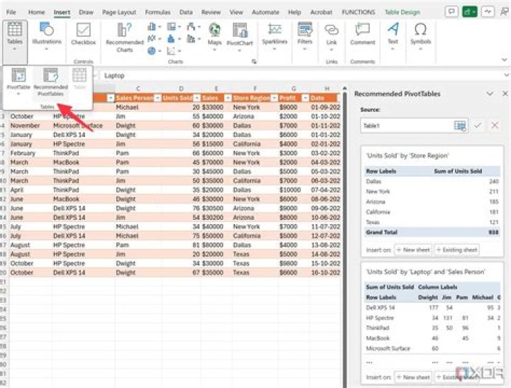
- STEP 1: Make sure you have selected your data. Go to Insert > Tables > Recommended Pivot Tables.
- STEP 2: You will see the generated Pivot Table recommendations.
- STEP 3: The generated Pivot Table is now in a new sheet. Let us make some changes to it.
- Helpful Resource:
How do I see recommended pivot tables Mac?
Pivot with a click Select your data table, then click Insert on the toolbar and then Recommended PivotTables in the Insert tab that appears.
What is the use of recommended pivot table in Excel?
Excel 2013 has a new feature Recommended PivotTables under the Insert tab. This command helps you to create PivotTables automatically. Step 1 − Your data should have column headers.What is the keyboard shortcut for recommended PivotTables?
PivotTable and PivotChart Wizard Keyboard Shortcut Use the keyboard shortcut Alt + D + P to open the PivotTable and PivotChart Wizard. This will take you through the steps to set up either a pivot table or pivot chart, select your data and the location for your new pivot table or chart.
How do you use the recommended Pivot Tables command to insert a blank pivot table in a new worksheet?
- Select the table or cells (including column headers) containing the data you want to use. …
- From the Insert tab, click the PivotTable command. …
- The Create PivotTable dialog box will appear. …
- A blank PivotTable and Field List will appear on a new worksheet.
How do I create a clustered pivot chart?
- Select any cell in the pivot table.
- On the Excel Ribbon, click the Insert Tab.
- In the Charts group, click Column, then click Clustered Column.
- A column chart is inserted on the worksheet, and it is selected — there are handles showing along the chart’s borders.
How do I edit a pivot table?
Edit a pivot table. Click anywhere in a pivot table to open the editor. Add data—Depending on where you want to add data, under Rows, Columns, or Values, click Add. Change row or column names—Double-click a Row or Column name and enter a new name.How do I add a calculated field to an attendance in a pivot table?
- Click the PivotTable. …
- On the Analyze tab, in the Calculations group, click Fields, Items, & Sets, and then click Calculated Field.
- In the Name box, type a name for the field.
- In the Formula box, enter the formula for the field. …
- Click Add.
- Select a field in the Values area for which you want to change the summary function of the PivotTable report.
- On the Options tab, in the Active Field group, click Active Field, and then click Field Settings. …
- Click the Summarize Values By tab.
How do I add a combination to a pivot chart in Excel?
- On the Insert tab, in the Charts group, click the Combo symbol.
- Click Create Custom Combo Chart.
- The Insert Chart dialog box appears. For the Rainy Days series, choose Clustered Column as the chart type. …
- Click OK. Result:
How do I add a filter to a pivot table?
- Click anywhere in the PivotTable to show the PivotTable tabs (PivotTable Analyze and Design) on the ribbon.
- Click PivotTable Analyze > Insert Slicer.
- In the Insert Slicers dialog box, check the boxes of the fields you want to create slicers for.
- Click OK.
How do I add a PivotTable to my keyboard?
Select the data set and press Alt > N > V (this is a sequential shortcut so press Alt then N then V). A dialog box will appear with options to create a pivot table.
How do you navigate a PivotTable using the keyboard?
ShortcutActionNotesCtrl + ASelect entire pivot table (not including Report Filters)Select Pivot Table Range
How do I resize a PivotTable?
- Right-click in the pivot table.
- Select Pivot Table Options.
- In the Pivot Table Options dialogue box, click the Layout and Format tab, and then uncheck the box Autofit column widths on update.
How do I count values in a PivotTable?
- Right-click on any cell in the ‘Count of Sales Rep’ column.
- Click on Value Field Settings.
- In the Value Field Settings dialog box, select ‘Distinct Count’ as the type of calculation (you may have to scroll down the list to find it).
- Click OK.
How do I add a pivot table to an existing worksheet?
- Click a cell in the source data or table range.
- Go to Insert > PivotTable. …
- Excel will display the Create PivotTable dialog with your range or table name selected. …
- In the Choose where you want the PivotTable report to be placed section, select New Worksheet, or Existing Worksheet.
How do I rerun a pivot table?
- Click anywhere in the PivotTable to show the PivotTable Tools on the ribbon.
- Click Analyze > Refresh, or press Alt+F5. Tip: To update all PivotTables in your workbook at once, click Analyze > Refresh All.
Why can't I add a calculated field to a pivot table?
Drop the data into Excel into a table. If you try to pivot off this data, the calculated field will still be grayed out. BUT, if you make a dynamic range on the table and create a new pivot table that references the dynamic range of the table instead of the table itself, the calculated field will not be grayed out.
How do I add a calculated field in Access?
- Select the Fields tab, locate the Add & Delete group, and click the More Fields drop-down command. Clicking the More Fields drop-down command.
- Hover your mouse over Calculated Field and select the desired data type. …
- Build your expression. …
- Click OK.
How do I change pivot table data is average?
You can simply click on the arrow next to the Sum of Sales field mentioned in the Values Area and select Value Field Setting. In the Value Field Setting dialog box, Select Average in the Summarize value by and Click OK.
How do I change the Summarize values in a pivot table?
In the PivotTable, right-click the value field you want to change, and then click Summarize Values By. Click the summary function you want. Note: Summary functions aren’t available in PivotTables that are based on Online Analytical Processing (OLAP) source data. The sum of the values.
Can you change multiple value field settings in pivot table?
If you want to change multiple pivot table fields, you can change the function in the Value Fields Settings, just do the following steps: Step1: select one filed in your pivot table, and right click on it, and then choose Value Fields Settings from the dropdown menu list. And the Value Fields Settings dialog will open.
How do I change a pivot chart to a combination chart?
In the pivot chart, right-click on one of the Cookies columns. In the Change Chart Type dialog box, click the Line chart type, and click one of the Line subtypes, then click OK. The chart is now a combination chart, with columns for Bars, Crackers and Snacks, and a line for Cookies.
What is combo chart?
A combo chart is a combination of two column charts, two line graphs, or a column chart and a line graph. You can make a combo chart with a single dataset or with two datasets that share a common string field.
How do I use advanced filter in pivot table?
Whatever you want to filter your pivot tables by (in Jason’s situation, it’s type of beer), you’ll need to apply that as a filter. Click within your pivot table, head to the “Pivot Table Analyze” tab within the ribbon, click “Field List,” and then drag “Type” to the filters list.
How do I link a pivot table to a cell filter?
- Please select the cell (here I select cell H6) you will link to Pivot Table’s filter function, and enter one of the filter values into the cell in advance.
- Open the worksheet contains the Pivot Table you will link to cell.
How do I filter multiple items in a pivot table?
- Right-click a cell in the pivot table, and click PivotTable Options.
- Click the Totals & Filters tab.
- Under Filters, add a check mark to ‘Allow multiple filters per field. ‘
- Click OK.
How do I create a pivot table wizard?
To open the PivotTable and PivotChart Wizard, select any cell on a worksheet, then press Alt+D, then press P. That shortcut is used because in older versions of Excel, the wizard was listed on the Data menu, as the PivotTable and PivotChart Report command.
How do you quickly select data in a pivot table?
Hold down SHIFT and click, or hold down CTRL and click to select additional items within the same field. To cancel selection of an item, hold down CTRL and click the item.
How do I move multiple columns in a pivot table?
- Click any cell in the PivotTable. The PivotTable Fields pane appears. You can also turn on the PivotTable Fields pane by clicking the Field List button on the Analyze tab.
- Click and drag a field to the Rows or Columns area.
